(You can download this notebook here.)
(Jump to Section 10 for a summary of the covered topics.)
.libPaths("/data/R/library")
suppressMessages(library("dplyr"))
suppressMessages(library("plot.matrix"))
suppressMessages(library("ggplot2"))
suppressMessages(library("lme4"))
suppressMessages(library("rstan"))
suppressMessages(library("brms"))
Pretty woman, Yeah, yeah, yeah
Pretty woman, Look my way
Pretty woman, Say you'll stay... with me
'Cause I need you, I'll treat you right
Come with me, baby, Be mine tonight
Pretty woman, Don't walk away
Hey, O.K., If that's the way it must be, O.K.
I guess I'll go on home, It's late
There'll be tomorrow night...
(Roy Orbison, “Oh, Pretty Woman”)
Music, Prostitution, and Statistics
Imagine your bass guitar teacher gives you a song to practice, which has a fancy bassline.
It is sung by a male, who praises the habitus of a female conspecific or more likely an imaginative one. He fantasizes inviting her for sexual intercourse, but at first seems rejected. When he threatens to re-iterate his invitation the next day, the female returns; the ending of this phantasy is left open.
Acknowledged, I am being annoying to analyze popular songs like this. However, for instrument practice, I usually listen over and over, so there is no evading the text. Nor its meaning.
I often play bass for practice on my way to work, on the train. I arrive at Brussels North Station. My train enters at “perron 12”, which is located furthest to the East. It is difficult to not notice how many brothels there are in Aarschotstraat (if a phenomenon has a wikipedia page, it is probably true and probably famous). Shop window prostituiton. The density of economically sustainable etablissements of this sort in the area keeps astonishing me. “Ero Polis”, “Club Virgin”, “Touch and Go” - a most creative sector! (Personally, I do not think this agglomeration is due to proximity to the European Institutions - that band of trustworthy, honorable and wealthy politicians far away from home.)
|
|


When I stand on the train door passing by, I engage in the fun exercise of counting the abundance of prostitutes and customers; fittingly sound-tracked by “pretty woman”. No offense in my leisure statistics; acknowledged that prostitution certainly is hard work. I smile when workers occasionally sit in front of a brothel in bathrobe, smoking and talking. Evidence and reminder that those (un-)dressed-up ladies are very normal persons. “Normal”, in a sense that we should keep in mind that few linger there voluntarily. Even if they do, they will certainly not consider it their dream job. Since only very recently, sex workers in Belgium gained access to very basic social security rights.. Which seems fair and contemporary.
And in respect of this achievement, and inspired by my bass guitar and counting exercises, I thought it is worth applying some rigorous statistics on this bio-economical system.
In fact, the true system which prompted me was the research of Ioanna Gavriilidi, a former colleague at UAntwerpen, who is studying “the evolution of cognition and personality in lizards”. Her recent data is not published1, but induced the thoughts I formulate below.
Thank you, Ioanna, and I hope you don’t mind the curious analogy I chose to replace your unpublished lizards ;)
Simulated Data
structure
The true abundance of the ladies in the storefronts and their “lovers” on the street is difficult to measure on brief observations:
- My observation point on the train is quite remote.
- There is repeated observation of the same individuals, but I do not keep ID’s.
- There is temporal fluctuation in these places’ occupation.
- No way I could tell whether an apparently absent worker is on holiday or busy in the back office.
Hence, I will rather work on synthetic data.
Assume you conduct a hypothetical experiment, counting the brothel preference of a population of “suitors” (i.e. customers, translated by google translate), depending on work day.
This experiment gives us the following observable variables:
preference, which can be measured by a binary variable indicating whether a subject visits a given brothel on a given weekday, or not.brothel, a list of bordellos.weekday, an arbitrarily categorized proxy of temporal periodicity.subject, an imaginary identifier of the shy customer.

For connaisseurs: this is called a “hierarchical overlapping multifactor model”2.
Behold how easily we can fiddle some simulated dataset in R. First we need a few framing structures.
# The Experiment takes quite a long time,
# owing to the large uncertainty in binary measurements
experiment_duration <- 2^5 # weeks.
weekdays <- weekdays(as.Date(4,"1970-01-01", tz="GMT")+0:6)
brothels <- c(
    "The Velvet Hideaway",
    "The Secret Garden",
    "The Rosewood Retreat",
    "Whispers & Lace"
    ) # I do prefer the real names, but need to avoid copyright issues.

n_weekdays <- length(weekdays)
n_brothels <- length(brothels)
n_subjects <- 2^6

subjects <- paste("customer", sprintf("%02.0f", 1:n_subjects))
The Pimp, The Priest, and The Experiment
K. would also go, once a week, to see a girl called Elsa who worked as a waitress in a wine bar through the night until late in the morning. During the daytime she only received visitors while still in bed.
Central to the model below will be the preference matrix of customers per weekday (elsewhere called a “lattice of factors”, here weekday \(\times\) brothel).
Each customer has a different base preference for each brothel, and that depends on weekday.
As you might notice later, this is the tautological implementation of the central modeling paradigm below, and you are welcome to dispute my approach.
To add some spice to this already hot topic, I choose to set the probability to flat 0.1 on Mondays, independent of brothel (who would visit the place on Monday, anyways).
Also, there are a pimp and a priest, subjects who will help us to get a hold on subject intercepts by operating at the limits of logit transformation.
# basic input
preferences_input <- matrix(
  floor(100 * runif(n_brothels * n_subjects, min = 0., max = 1.))/100,
  nrow = n_subjects, byrow = TRUE
)

# let's give the data a very distinct weekday effect
weekday_modulation <- 1:n_weekdays / 5.0
weekday_modulation <- c(weekday_modulation[3:1], weekday_modulation[2:5])

# along the same line, brothels increase in popularity the closer they are to the station (unquantified)
brothel_modulation <- 1:n_brothels / (4*n_brothels) + 0.75

# empty data storage
data <- data.frame()

# preference matrix for reference
preference_matrix_theoretical <- array(, c(n_weekdays, n_brothels, n_subjects))
preference_matrix_theoretical[,,] <- 0

# brothel visits, /in silico/
for (i in 1:n_subjects) {
  for (br in 1:n_brothels) {
    for (wd in 1:n_weekdays) {
      prob <- preferences_input[i, br] * weekday_modulation[wd] * brothel_modulation[br]

      # The Monday Dip
      if (wd == 1){
        prob <- 0.1
      }

      # The Pimp: visiting every brothel every day.
      if (i == 1){
        prob <- 1.0
      }

      # The Priest: never seen around Aarschotstraat.
      if (i == n_subjects){
        prob <- 0.0
      }

      # store true probability for ex post comparison
      preference_matrix_theoretical[wd, br, i] <-
        preference_matrix_theoretical[wd, br, i] + prob

      # The Experiment: here we flip a coin.
      experiment <- data.frame(
        "visit" = rbinom(experiment_duration, size = 1, prob = prob)
      )

      # meta data
      experiment$subject <- subjects[i]
      experiment$weekday <- weekdays[wd]
      experiment$brothel <- brothels[br]

      data <- rbind(data, experiment)
      # data <- bind_rows(data, experiment)
    }
  }
}

# re-arrange columns
data <- data[, c(2:ncol(data), 1)]

# data formats
data$subject <- factor(data$subject)
data$brothel <- factor(data$brothel, levels = brothels)
data$weekday <- factor(data$weekday, levels = weekdays)

# behold: the data
knitr::kable(data[sample(nrow(data), 5), ])
| subject | weekday | brothel | visit | |
|---|---|---|---|---|
| 5667 | customer 07 | Wednesday | The Secret Garden | 1 |
| 12802 | customer 15 | Tuesday | The Secret Garden | 0 |
| 23324 | customer 27 | Monday | The Velvet Hideaway | 0 |
| 28388 | customer 32 | Saturday | The Rosewood Retreat | 0 |
| 56829 | customer 64 | Friday | The Secret Garden | 0 |
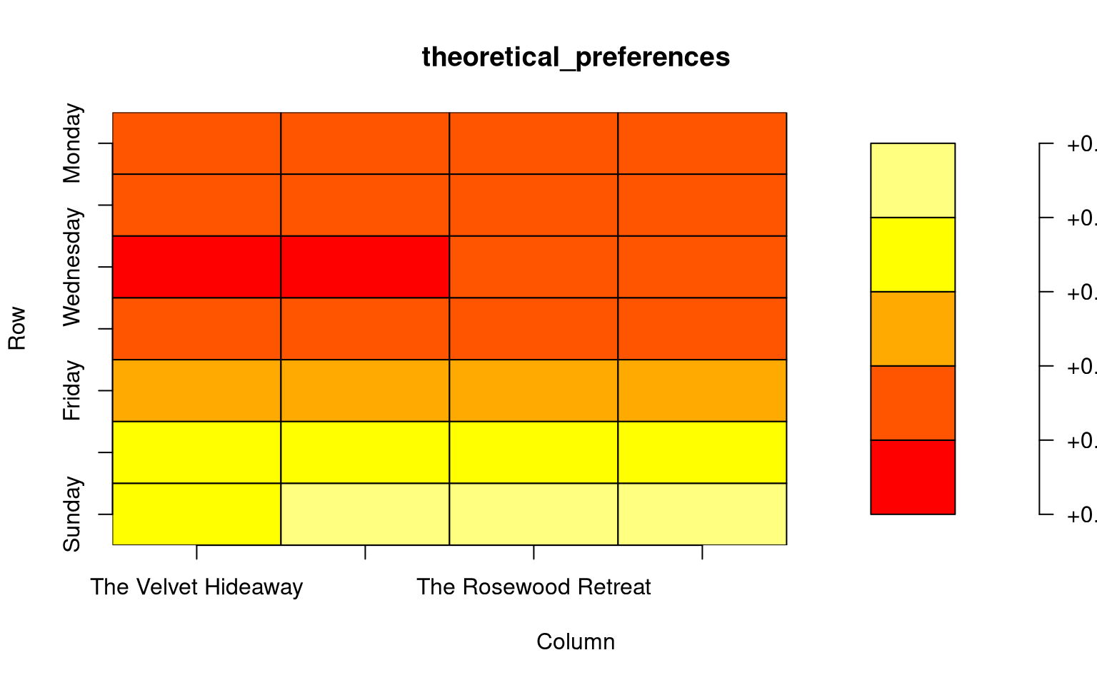
The theoretical patterns look like this (ref):
theoretical_preferences <- apply(preference_matrix_theoretical, MARGIN=c(1, 2), sum) / n_subjects

rownames(theoretical_preferences) <- weekdays
colnames(theoretical_preferences) <- brothels
plot(theoretical_preferences) # using plot.matrix
The patterns we put into the data should be visible in the data.
data %>%
  group_by(brothel, weekday) %>%
  summarize(visit = sum(visit)) %>%
  ggplot(aes(x = brothel, y = weekday, fill = visit)) +
  geom_tile() +
  scale_y_discrete(limits = rev) +
  theme_bw() +
  theme(legend.position = "none")
`summarise()` has grouped output by 'brothel'. You can override using the
`.groups` argument.
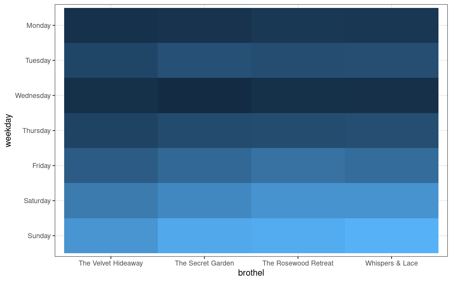
(Take good note of the differences between these two heatmaps…)
Observing all combinations of parameters is impossible in the research on red light and trenchcoats. Here is a simple function to subsample, which one could use to perform a sort of power analysis.
subsample <- function(percentage) {
  assertthat::assert_that(
    is.numeric(percentage) &&
    (0.0 <= percentage) &&
    (percentage <= 1.0),
    msg = "Percentage must be numeric between 0.0 and 1.0.")
  sub_n <- as.integer(round(nrow(data)*percentage, 0))
  return(data[sample(nrow(data), sub_n, replace = FALSE), ])
}
knitr::kable(subsample(7/nrow(data)))
| subject | weekday | brothel | visit | |
|---|---|---|---|---|
| 449 | customer 01 | Monday | The Rosewood Retreat | 1 |
| 21298 | customer 24 | Monday | Whispers & Lace | 0 |
| 454 | customer 01 | Monday | The Rosewood Retreat | 1 |
| 50582 | customer 57 | Saturday | The Secret Garden | 0 |
| 35726 | customer 40 | Thursday | Whispers & Lace | 0 |
| 34651 | customer 39 | Friday | The Rosewood Retreat | 0 |
| 8395 | customer 10 | Thursday | The Secret Garden | 0 |
Table 1: Subsampling the dataset. This is a very small subset.
The Naïve Model
model fitting
The effects above seem pretty simple, right? Visit rate is affected by weekday, brothel, and subject; the latter might best justify a random intercept.
You might struggle with the “family”, but it is something along the lines of beta binomial or Bernoulli. Should be trivial to get our input effects back, we know what the result should be.
There is nothing wrong about GOogling Good Old Generalized Linear Models (“Go, go, GLM!™”)3. There are numerous texts and tutorials online, which you can easily reproduce. For a start, we use “Wilkinson Notation”4, i.e. formulas, as any sane person would (right?).
fit_glm <- function(formula_str){
  stats::glm(
    formula = as.formula(formula_str),
    data = subsample(1.),
    family = binomial(link = 'logit')
  )
}
Fire ahead, using stats::glm on the complete data set.
naive_model <- fit_glm("visit ~ brothel + weekday")
summary(naive_model)
Call:
stats::glm(formula = as.formula(formula_str), family = binomial(link = "logit"),
    data = subsample(1))

Coefficients:
                            Estimate Std. Error z value Pr(>|z|)
(Intercept)                 -2.16746    0.03912 -55.412  < 2e-16 ***
brothelThe Secret Garden     0.14894    0.02945   5.058 4.25e-07 ***
brothelThe Rosewood Retreat  0.22463    0.02922   7.688 1.50e-14 ***
brothelWhispers & Lace       0.22948    0.02921   7.857 3.92e-15 ***
weekdayTuesday               0.55967    0.04441  12.603  < 2e-16 ***
weekdayWednesday            -0.20472    0.05055  -4.050 5.13e-05 ***
weekdayThursday              0.51444    0.04466  11.518  < 2e-16 ***
weekdayFriday                1.02389    0.04237  24.167  < 2e-16 ***
weekdaySaturday              1.45115    0.04129  35.144  < 2e-16 ***
weekdaySunday                1.75932    0.04091  43.008  < 2e-16 ***
---
Signif. codes:  0 '***' 0.001 '**' 0.01 '*' 0.05 '.' 0.1 ' ' 1

(Dispersion parameter for binomial family taken to be 1)

    Null deviance: 62769  on 57343  degrees of freedom
Residual deviance: 58374  on 57334  degrees of freedom
AIC: 58394

Number of Fisher Scoring iterations: 4
Great, all so significant! (Except on Wednesday.)
At this point, Some would rush to publish a paper. I would not. There are at least two immediate annoyances for me personally:
- We left data space for
logit. This needs to be translated back, otherwise numbers as “the intercept” are meaningless. - The model output comes with an intercept and differential effects. The intercept is “Monday” in a certain brothel.
All weekdays are equal, but some weekdays are more equal than others.
(Modified, from “Animal Farm”.)
data transformation: There and back again…
How can we interpret that? See here!
\( log\left(\frac{p}{1-p}\right) = \beta_0 + \sum\limits_i \beta_i x_i \)
But.. wait… this will leave x in the calculation for p.
See here!
We cannot really convert back.
Yet it works punctually, e.g. on the intercept. Let us simplify \(\xi = exp\left(\beta_0 + \beta_1\cdot x_1 + …\right)\)
\( p = \xi - p \cdot \xi \)
\( p \cdot (1 + \xi ) = \xi \)
\( p = \frac{\xi}{1 + \xi} \)
This can give a computer formula:
# the inversion of log odds
oggLods <- function (xi) exp(xi) / (1 + exp(xi) )

# calculation for the intercept
oggLods( naive_model$coefficients["(Intercept)"] )
(Intercept)
  0.1027112
theoretical_preferences[1, 1]
[1] 0.1125
# ... or for "brothelThe Secret Garden" on "weekdayWednesday"
oggLods(
  naive_model$coefficients["(Intercept)"] +
  naive_model$coefficients["brothelThe Secret Garden"] +
  naive_model$coefficients[paste0("weekday", weekdays[3], collapse = "")]
)
(Intercept)
 0.09768349
theoretical_preferences[2, 3]
[1] 0.1924609
Unfortunately, no good match, although sample size is extraordinary. Maybe the other way round? After all, we know the input probabilities!
Here is the well-known transfer function, by the way:
p_log <- function (p) log(p / (1-p))

x <- seq(0., 1., length.out = 101)
plot(p_log(x), x, type = 'l')
![Figure 4: The logit function maps the \left[ 0, 1\right] interval to \left[ -\infty, +\infty\right].](/images/39.lattice_models/fig-logit-1.png)
We have to account for the fact that the naïve model only gives differences from the intercept.
# comparing the real and modeled Secret Garden slope on Wednesdays...

p_log(theoretical_preferences[3, 2]) - p_log(theoretical_preferences[3, 1])
[1] 0.08896846
naive_model$coefficients["brothelThe Secret Garden"]
brothelThe Secret Garden
                0.148945
No good.
The model converged. Significances pop out. No warning signs by the modeling library. However, the model outcome does not match the data input probabilities of the simulated data.
Yes, you should be concerned. Your model is wrong.
Let’s keep the comparison, anyways: we don’t know yet whether the model or the transformation were a mismatch.
And, now, take a piece of paper and note some reference numbers, to hopefully match later models:
- The log probability for “The Velvet Hideaway” on Monday is -2.07 (calculation: “intercept”).
- The log probability for “The Velvet Hideaway” on Sunday is -0.42 (calculation: “intercept + Sunday”).
- The log probability for “The Rosewood Retreat” on Monday is -2.07 (calculation: “intercept + rosewood”).
- The log probability for “The Secret Garden” on Thursday is -1.49 (calculation: “intercept + Thursday + garden”).
- The Pimp certainly comes around,
p_log: Inf. - The Priest certainly not, thus
p_log: -Inf.
The Bayesian Model
Introducing brms
Okay, okay, maybe “Go, go, GLM!™” was not the right slogan. Everyone fancies Bayesian statistics nowadays. And “Mixed Models”: you of course noticed that we forgot the subject intercept above.
Hang on, here is your friendly library to solve it: brms (as in “BRiMStone”, in reference to the smoothness of its compiling and sampling procedure).
Documentation is abundant …
We may use formulas as above. Note that the family is “Bernoulli” this time. WTF, should we maybe have called to Brother Bernoulli in the first place?
If, as I do, you have trouble formulating the correct formulas for you statistical question, put more effort to find books and guides online, and “never give up”.
Anyways. To keep settings consistent during this test, a function wrapper will be useful.
fit_brms_model <- function(formula_str) {
  brms::brm(
    formula = as.formula(formula_str),
    data = subsample(1.),
    family = bernoulli(link = 'logit'),
    chains = 2,
    iter = 2^11,
    cores = 2
  )
}
Pretty easy going, just much more work for the computer.
brms_model <- fit_brms_model("visit ~ brothel + weekday")
Compiling Stan program...

Start sampling
summary(brms_model)
# plot(brms_model)
This one is perfectly consistent with stats::glm, and therefore wrong.
There is added value (will come clear below) and added sampling duration by switching to the Bayesian approach.
Random Intercepts: Pimp and Priest Revisited
Though this may have worked technically, we yet have to prove that we can recover our Pimp and Priest.
This goes by a random intercept, appended to the model as follows:
# This chunk is NOT evaluated, to save my precious lifetime.
random_intercept_model <- fit_brms_model("visit ~ brothel + weekday + (1|subject)")
summary(random_intercept_model)
Sampling is creeping slow, which might not be the best symptom. Usually, sampling speed increases with setting good priors. Conversely, it decreases with sample size. I also think that Pimp and Priest are show stoppers, because they are on the far ends of the sampling space, and more than half of the sampler iterations are discarded because one of them leaves the sampling space.
Back to Frequentist Frameworks!
Model Formula Exploration
Yet Another Modeling Library
Model formulas are a science by itself. It is worth spending some time to find the right one.
It turns out that stats::glm is not capable of using factor-type random intercepts.
There are a gazilion other packages for linear mixed models, and I randomly chose lme4 (documentation, documentation, documentation).
There is documentation online.
fit_glmer <- function(formula_str) {
  lme4::glmer(
    formula = as.formula(formula_str),
    data = subsample(1.),
    family = binomial(link = 'logit')
  )
}
One Random Intercept
The subject effect is certainly one of interest; we model a random intercept.
random_intercept_model <- fit_glmer("visit ~ brothel + weekday + (1|subject)")
coef(random_intercept_model)$'subject'$'(Intercept)'
 [1]  4.414869 -2.181079 -2.607098 -2.293659 -1.705174 -1.846410 -2.048623
 [8] -2.514704 -2.314098 -2.320952 -1.910402 -1.928077 -2.123494 -2.671277
[15] -2.376553 -1.812010 -2.079568 -2.155326 -3.105557 -1.898674 -2.383603
[22] -2.155326 -3.895396 -2.507197 -2.869705 -1.705174 -2.433612 -2.529803
[29] -2.383603 -2.092045 -2.720926 -2.161739 -1.789262 -2.695931 -2.646950
[36] -2.355538 -1.875343 -1.910402 -2.679458 -2.200569 -3.105557 -2.440853
[43] -2.455412 -2.729335 -2.704224 -2.104580 -2.492266 -2.142546 -3.607858
[50] -2.048623 -2.054784 -3.116199 -2.060959 -1.738589 -2.098305 -2.181079
[57] -1.761026 -2.174616 -2.869705 -2.833521 -2.815715 -3.181680 -3.464298
[64] -6.796103
There seem to be a Priest and a Pimp.
How about the so-called “fixed” effects (which are really just random parameters)?
summary(random_intercept_model)
Generalized linear mixed model fit by maximum likelihood (Laplace
  Approximation) [glmerMod]
 Family: binomial  ( logit )
Formula: visit ~ brothel + weekday + (1 | subject)
   Data: subsample(1)

      AIC       BIC    logLik -2*log(L)  df.resid
  53751.3   53849.8  -26864.6   53729.3     57333

Scaled residuals:
    Min      1Q  Median      3Q     Max
-1.2739 -0.5431 -0.3720 -0.0845  7.0125

Random effects:
 Groups  Name        Variance Std.Dev.
 subject (Intercept) 1.286    1.134
Number of obs: 57344, groups:  subject, 64

Fixed effects:
                            Estimate Std. Error z value Pr(>|z|)
(Intercept)                 -2.35291    0.14792 -15.906  < 2e-16 ***
brothelThe Secret Garden     0.16466    0.03095   5.320 1.04e-07 ***
brothelThe Rosewood Retreat  0.24808    0.03070   8.081 6.44e-16 ***
brothelWhispers & Lace       0.25342    0.03068   8.259  < 2e-16 ***
weekdayTuesday               0.62947    0.04724  13.325  < 2e-16 ***
weekdayWednesday            -0.23885    0.05461  -4.373 1.22e-05 ***
weekdayThursday              0.57947    0.04752  12.193  < 2e-16 ***
weekdayFriday                1.13774    0.04504  25.261  < 2e-16 ***
weekdaySaturday              1.60162    0.04395  36.441  < 2e-16 ***
weekdaySunday                1.93586    0.04361  44.394  < 2e-16 ***
---
Signif. codes:  0 '***' 0.001 '**' 0.01 '*' 0.05 '.' 0.1 ' ' 1

Correlation of Fixed Effects:
            (Intr) brtTSG brtTRR brtW&L wkdyTs wkdyWd wkdyTh wkdyFr wkdySt
brthlThScrG -0.110
brthlThRswR -0.112  0.523
brthlWhsp&L -0.112  0.523  0.528
weekdayTsdy -0.194  0.002  0.003  0.003
wekdyWdnsdy -0.168  0.000 -0.001 -0.001  0.524
wekdyThrsdy -0.193  0.002  0.003  0.003  0.603  0.521
weekdayFrdy -0.204  0.004  0.007  0.007  0.636  0.550  0.632
weekdyStrdy -0.210  0.007  0.011  0.011  0.652  0.563  0.648  0.685
weekdaySndy -0.213  0.009  0.015  0.015  0.658  0.568  0.654  0.691  0.710
knitr::kable(fixef(random_intercept_model))
| x | |
|---|---|
| (Intercept) | -2.3529117 |
| brothelThe Secret Garden | 0.1646556 |
| brothelThe Rosewood Retreat | 0.2480837 |
| brothelWhispers & Lace | 0.2534217 |
| weekdayTuesday | 0.6294676 |
| weekdayWednesday | -0.2388457 |
| weekdayThursday | 0.5794682 |
| weekdayFriday | 1.1377431 |
| weekdaySaturday | 1.6016182 |
| weekdaySunday | 1.9358564 |
Maybe interaction terms help?
Interaction Terms
Interaction terms, in the current example, are describing the combined effect of brothel and weekday.
For example: the overall log visit rate of “The Velvet Hideaway” versus “Whispers & Lace” might be \(+1.0\) on Wednesdays, but it is \(\pm 0.0\) on Mondays and maybe \(+2.0\) on Sundays.
In general terms, the magnitude of one effect varies depending on another parameter.
This is put into formula with the term brothel:weekday.
Note that this is order dependent, brothel:weekday \(\neq\) weekday:brothel.
As an extra confusion convenience, brothel * weekday is equivalent to brothel + weekday + brothel:weekday (non-commutative).
And even more implicit useful when you have more than three parameters, brothel * weekday - weekday is equivalent to brothel + brothel:weekday.
And, why not, you could even do brothel / weekday.
I wonder whether Wilkinson5 knew what he did to us.
There are more formula variants for your specific modeling needs (see also here and here).
Here, we can probably use the full interaction.
interaction_model <- fit_glmer("visit ~ brothel + weekday + brothel:weekday + (1|subject)")
Warning in checkConv(attr(opt, "derivs"), opt$par, ctrl = control$checkConv, :
Model failed to converge with max|grad| = 0.00305197 (tol = 0.002, component 1)
# summary(interaction_model)
coef(interaction_model)$'subject'$'(Intercept)'
 [1]  4.459104 -2.136665 -2.562968 -2.249319 -1.660490 -1.801797 -2.004126
 [8] -2.470511 -2.269771 -2.276629 -1.865824 -1.883509 -2.079044 -2.627190
[15] -2.332267 -1.767379 -2.035090 -2.110895 -3.061746 -1.854089 -2.339322
[22] -2.110895 -3.851974 -2.462999 -2.825748 -1.660490 -2.389364 -2.485621
[29] -2.339322 -2.047575 -2.676872 -2.117313 -1.744619 -2.651861 -2.602847
[36] -2.311239 -1.830746 -1.865824 -2.635377 -2.156168 -3.061746 -2.396611
[43] -2.411180 -2.685287 -2.660159 -2.060118 -2.448058 -2.098107 -3.564315
[50] -2.004126 -2.010291 -3.072395 -2.016470 -1.693920 -2.053839 -2.136665
[57] -1.716369 -2.130198 -2.825748 -2.789541 -2.771723 -3.137914 -3.420686
[64] -6.753258
knitr::kable(fixef(interaction_model))
| x | |
|---|---|
| (Intercept) | -2.3085625 |
| brothelThe Secret Garden | 0.0749153 |
| brothelThe Rosewood Retreat | 0.2188432 |
| brothelWhispers & Lace | 0.1983544 |
| weekdayTuesday | 0.6049465 |
| weekdayWednesday | -0.0676528 |
| weekdayThursday | 0.5380133 |
| weekdayFriday | 1.0518275 |
| weekdaySaturday | 1.5237285 |
| weekdaySunday | 1.8548648 |
| brothelThe Secret Garden:weekdayTuesday | 0.1580597 |
| brothelThe Rosewood Retreat:weekdayTuesday | -0.0472032 |
| brothelWhispers & Lace:weekdayTuesday | -0.0128779 |
| brothelThe Secret Garden:weekdayWednesday | -0.2872227 |
| brothelThe Rosewood Retreat:weekdayWednesday | -0.2252158 |
| brothelWhispers & Lace:weekdayWednesday | -0.1734339 |
| brothelThe Secret Garden:weekdayThursday | 0.1179732 |
| brothelThe Rosewood Retreat:weekdayThursday | -0.0081913 |
| brothelWhispers & Lace:weekdayThursday | 0.0540084 |
| brothelThe Secret Garden:weekdayFriday | 0.1287882 |
| brothelThe Rosewood Retreat:weekdayFriday | 0.1389892 |
| brothelWhispers & Lace:weekdayFriday | 0.0666164 |
| brothelThe Secret Garden:weekdaySaturday | 0.0955222 |
| brothelThe Rosewood Retreat:weekdaySaturday | 0.0923180 |
| brothelWhispers & Lace:weekdaySaturday | 0.1172774 |
| brothelThe Secret Garden:weekdaySunday | 0.1478082 |
| brothelThe Rosewood Retreat:weekdaySunday | 0.0446608 |
| brothelWhispers & Lace:weekdaySunday | 0.1270735 |
Ignoring the convergence error, you might consider this a reasonably complex model, sweatily write a methods section, report the significant outcomes, and rush to Nature to publish.
Only problem: the outcome is not quite right yet.
Multiple Random Intercepts (\(MRI^{TM}\))
Instead of considering the different brothels as slopes, you might consider them as another “random” intercept.
Why not, let’s go “all in”:
all_intercept_model <- fit_glmer("visit ~ (1|brothel:weekday) + (1|subject)")
summary(all_intercept_model)
Generalized linear mixed model fit by maximum likelihood (Laplace
  Approximation) [glmerMod]
 Family: binomial  ( logit )
Formula: visit ~ (1 | brothel:weekday) + (1 | subject)
   Data: subsample(1)

      AIC       BIC    logLik -2*log(L)  df.resid
  53879.0   53905.9  -26936.5   53873.0     57341

Scaled residuals:
    Min      1Q  Median      3Q     Max
-1.2924 -0.5420 -0.3716 -0.0852  6.9655

Random effects:
 Groups          Name        Variance Std.Dev.
 subject         (Intercept) 1.2995   1.1400
 brothel:weekday (Intercept) 0.5672   0.7531
Number of obs: 57344, groups:  subject, 64; brothel:weekday, 28

Fixed effects:
            Estimate Std. Error z value Pr(>|z|)
(Intercept)  -1.3792     0.2018  -6.834 8.25e-12 ***
---
Signif. codes:  0 '***' 0.001 '**' 0.01 '*' 0.05 '.' 0.1 ' ' 1
attributes(coef(all_intercept_model))
$names
[1] "subject"         "brothel:weekday"

$class
[1] "coef.mer"
coef(all_intercept_model)$'subject'$'(Intercept)'
 [1]  5.3915446 -1.2076594 -1.6334734 -1.3201712 -0.7321787 -0.8732647
 [7] -1.0752990 -1.5411116 -1.3405984 -1.3474486 -0.9371961 -0.9548545
[13] -1.1501141 -1.6976341 -1.4030209 -0.8388998 -1.1062203 -1.1819232
[19] -2.1318501 -0.9254784 -1.4100674 -1.1819232 -2.9218102 -1.5336075
[25] -1.8960197 -0.7321787 -1.4600532 -1.5562054 -1.4100674 -1.1186878
[31] -1.7472695 -1.1883327 -0.8161754 -1.7222816 -1.6733138 -1.3820170
[37] -0.9021701 -0.9371961 -1.7058129 -1.2271370 -2.1318501 -1.4672916
[43] -1.4818442 -1.7556769 -1.7305724 -1.1312136 -1.5186828 -1.1691524
[49] -2.6341951 -1.0752990 -1.0814555 -2.1424919 -1.0876258 -0.7655560
[55] -1.1249434 -1.2076594 -0.7879688 -1.2012006 -1.8960197 -1.8598416
[61] -1.8420387 -2.2079724 -2.4906115 -5.8310981
modeled_logit_preferences <- matrix(coef(all_intercept_model)$'brothel:weekday'$'(Intercept)', nrow = n_weekdays, ncol = n_brothels)
rownames(modeled_logit_preferences) <- weekdays
colnames(modeled_logit_preferences) <- brothels

reference_logit_preferences <- p_log(theoretical_preferences)

knitr::kable(modeled_logit_preferences - reference_logit_preferences)
| The Velvet Hideaway | The Secret Garden | The Rosewood Retreat | Whispers & Lace | |
|---|---|---|---|---|
| Monday | -0.2321699 | -0.1581604 | -0.0165473 | -0.0366075 |
| Tuesday | -0.1012886 | 0.0234630 | -0.0959519 | -0.0973106 |
| Wednesday | -0.0727636 | -0.3691729 | -0.2168351 | -0.1987640 |
| Thursday | -0.1676975 | -0.0826678 | -0.1236974 | -0.0973106 |
| Friday | -0.1277861 | -0.0466484 | 0.0392312 | -0.0705559 |
| Saturday | -0.0364034 | -0.0048810 | 0.0575088 | 0.0418119 |
| Sunday | -0.0392208 | 0.0238258 | -0.0261190 | 0.0118532 |
This is the best example so far. And that is no surprise: the model formula kind of matches the data generation.
Tip
What we learned:
- We can use multiple intercept blocks in one model (which you might find confusing).
- The
(1|brothel:weekday)gives us a sort of matrix of intercept effects (see below), which might be accurate in cases when every parameter combination has their own intercept (and sampling size is sufficient to infer all these parameters).
The “i” in brms stands for “instructive”.
Double check: the same works in brms.
all_intercept_brm <- fit_brms_model("visit ~ (1|brothel:weekday) + (1|subject)")
Compiling Stan program...

Start sampling

Warning: Bulk Effective Samples Size (ESS) is too low, indicating posterior means and medians may be unreliable.
Running the chains for more iterations may help. See
https://mc-stan.org/misc/warnings.html#bulk-ess

Warning: Tail Effective Samples Size (ESS) is too low, indicating posterior variances and tail quantiles may be unreliable.
Running the chains for more iterations may help. See
https://mc-stan.org/misc/warnings.html#tail-ess
# fixef(all_intercept_brm) # the intercept
# head(coef(all_intercept_brm)$'subject', 3) # the pimp
# tail(coef(all_intercept_brm)$'subject', 3) # the priest

# or, get the info in matrix form:
coeffs <- coef(all_intercept_brm)$'brothel:weekday'
coeffs <- data.frame(coeffs)[,1]
coeffs <- matrix(coeffs, nrow = n_weekdays, ncol = n_brothels)
rownames(coeffs) <- sort(weekdays)
colnames(coeffs) <- sort(brothels)
brm_logit_preferences <- coeffs[weekdays,][,brothels]

knitr::kable(brm_logit_preferences - reference_logit_preferences)
| The Velvet Hideaway | The Secret Garden | The Rosewood Retreat | Whispers & Lace | |
|---|---|---|---|---|
| Monday | -0.2135638 | -0.1399100 | 0.0021611 | -0.0174091 |
| Tuesday | -0.0816053 | 0.0424871 | -0.0769057 | -0.0789890 |
| Wednesday | -0.0585850 | -0.3543203 | -0.2000627 | -0.1805641 |
| Thursday | -0.1484516 | -0.0629855 | -0.1051925 | -0.0781088 |
| Friday | -0.1082455 | -0.0255760 | 0.0589995 | -0.0509734 |
| Saturday | -0.0160549 | 0.0147105 | 0.0788439 | 0.0626817 |
| Sunday | -0.0180642 | 0.0462002 | -0.0038650 | 0.0330890 |
Very slow to sample, yet about as accurate as the above. Nice.
We can read the stancode of the model above:
stancode(all_intercept_brm)
Okay - wait a second.
Wasn’t our fear of stan syntax the reason to choose brms in the first place?
Why should we do this?
Do not fret. We might learn a thing or two.
stan_code <- brms::make_stancode("visit ~ (1|brothel:weekday) + (1|subject)", data = data)

fi <- file("multi_intercept_model_brm.stan")
writeLines(stan_code, fi)
close(fi)
In case you cannot guess, stancode() and make_stancode() will give you the stan code that was internally used by brms and rstan to represent the model you specified in the formula.
Take a second to read that model code! Remember your personal answer to the following questions.
- Could you have guessed that
Stan-code from the model formula? - Could you report the model structure (i.e. what exactly you model) in a “Methods” paragraph?
Optionally prune and alter the formula and re-iterate the reading exercise.
I personally learn two things:
- That I am almost unable (and, to some degree, unwilling) to understand what they are doing. The model formula is generic, not necessarily efficient, probably inflexible.
- From what I read in the Stan export, I would be unable to communicate my model structure in human language.
Acknowledged: brms never intended to provide a formula bespoke for our test problem.
It is created to be generic.
Let me give you a more bespoke Stan model for our prostitution example.
Enter The Matrix: Stan!
Feature Overview
The main characteristics of Stan are:
C-like syntax for variable definition- rigorous a priori data type declaration
- distinct program blocks for specific purposes
- separate model compilation and sampling (program execution)
You might love or hate those: using Stan directly instead of its derivatives gives you a lot of power, at the price of some code tinkering headache (which fades over time).
I will slowly walk through the blocks of code.
You might find the distinction of blocks confusing.
As I understand it, those blocks give context to the model code:
because of them, the compiler knows which variable to place or report where.
For example, data are observed variables submitted by the user, parameters are to be tuned by sampling, model contains the model definition and calculation specificities (with parameters not reported to the user).
Note that I did not originally intend this model to become so complex. I started small, ran into problems, learned something, and expanded. That is a usual experience on modeling.
Data Block
Let me give you, and explain, a possible data block for our problem.
The “data” block is quite trivial, though cumbersome: It defines all kinds of sample size parameters, along with empty vectors to hold the observed data.
Refer to the in-code comments for details.
stan_data_block <- "
  int n; // number of observations in the data
  int<lower = 0, upper = 1> y[n]; // integer of length n for outcome ('visit')

  // we use auxiliary observations to steer the sampler with the various intercepts (explained below)
  int<lower = 0, upper = 1> y_aux[n]; // integer of length n_aux for auxiliary outcome

  int n_subjects; // number of subjects
  array[n] int<lower=1, upper=n_subjects> subject_observed;  // vector of length n for subject id of each observation

  int n_weekdays; // number of weekdays
  array[n] int<lower=1, upper=n_weekdays> weekday_observed;  // vector of length n for actual weekdays

  int n_brothels; // number of different brothels
  array[n] int<lower=1, upper=n_brothels> brothel_observed;  // vector of length n for observed brothels
"
Parameters Block
Next is an interesting one, the parameters block.
Again, lots of data types and initially empty variables. However, this time, the variables are not supposed to be filled with data. These will be the estimated model parameters of interest.
stan_parameters_block <- "
  real population_intercept; // a population level intercept for the subjects
  real<lower = 0> population_variation; // variation of subjects around the intercept
  vector[n_subjects] subject_intercept; // (random) intercept per subject, to be sampled from the population_intercept

  matrix[n_weekdays, n_brothels] preferences; // the preference matrix, with weekdays in rows and brothels in columns
"
Do you recognize the preference matrix? It is to be filled with the preferences of the “suitors” for a given brothel, per weekday.
By now it contains meaningless data. Next step, in the model block, it will receive prior values. Finally, upon sampling, it will be tuned to the actual data. This is the life cycle of every Bayesian modeling parameter.
The subject_intercept, on the other hand, is the random intercept: a classical hierarchical parameter, sampling parametrization.
Subjects will be associated with a personal intercept value, all of which are sampled from a higher level (Normal) distribution with population_intercept as the mean and pupulation_variation as the sigma/spread/standard deviation.
In addition to the plain parameters, we can give Stan a block of transformed parameters.
Those are derived quantities which can be directly calculated from data and parameters.
The calculation is done on every sampling iteration, which means we get a trace of them, which is to say that we can report their outcome in that most valuable distribution form.
Here, I use transformed parameters to optionally center the subject factor and the preference matrix, aggregating their means on a “global intercept”.
stan_trafo_block <- "

  // intercept per subject, relative to population intercept
  vector[n_subjects] subject_intercept_centered = subject_intercept - population_intercept;

  // the preference matrix, centered
  real preferences_mean = mean(preferences);
  matrix[n_weekdays, n_brothels] preferences_centered = preferences - preferences_mean;

  // a global intercept aggregating the sum of the means of the other intercepts
  // (you might call it 'baseline preference')
  real global_intercept = population_intercept + preferences_mean;

"
Model Block
The model block, finally, the heart of our efforts.
It can contain more variable declarations (usually temporary helper variables), but those are not reported.
stan_model_block <- "

  // population intercept, priors
  population_intercept ~ normal(-1.2, 1.0); // population level mean
  population_variation ~ cauchy( 0.0, 1.0); // variation across individuals

  // subject intercept: one base preference for each individual
  for (i in 1:n_subjects) {
    subject_intercept[i] ~ normal(population_intercept, population_variation);
    // each subject is sampled from a 'Normal', the shape of which will be inferred during sampling.
    // Note that the Pimp and Priest sabotage this, or the other way round.
  }

  // prior for the preference matrix
  for (i in 1:n_weekdays) {
    for (j in 1:n_brothels) {
      preferences[i, j] ~ normal(0.0, 1.0);
    }
  }

  // for each observation, we select the corresponding matrix field
  //   and thereby add only one specific effect component for each data row
  vector[n] preference_per_observation; // a data-shaped vector of preferences, comprised by elements of the preference matrix
  for (i in 1:n) {
    preference_per_observation[i] = preferences[weekday_observed[i], brothel_observed[i]];
    // e.g. if the first observation was the first brothel on Monday, it will get the upper left value of the preference matrix.
  }

  // 'likelihood' / 'posterior'

  // pre-condition the relative subject preferences with auxiliary data (see text)
  y_aux ~ bernoulli_logit(subject_intercept[subject_observed]);

  // linear equation: subject intercept + preference
  y ~ bernoulli_logit(subject_intercept[subject_observed] + preference_per_observation);

"
The first part herein is the definition of the “random” intercept, i.e. an individual starting point for the preference of each “suitor”.
On initial attempts, I experienced sampling issues, which manifested in slow sampling and non-stationary trace plots6.
If defining the model without the y_aux auxiliary data, the sampler can distribute variation freely between the “population intercept” (i.e. factor subject) and the mean of the preference matrix (i.e. preferences_mean).
Note that I attempted to soft-constrain the random intercept to average out to zero, yet this did not work reliably. A loose prior as used above would normally allow the sampler to shift the intercept back and forth between the population intercept (subject factor) and the mean of the preference matrix (the other factors). The model is a bit ill-defined: the jargon terms are “identifiability” and “degeneracy”.
To cope with identifiability, the “auxiliary observations” are introduced. Those are extra samples of only one of the given factors7, in our case, subject, to facilitate the variability allocation of the sampler and support convergence. Having multiple “posterior” blocks in succession will keep the subject intercepts close to their global average, shifting the largest component of non-centered variation to subject factor. Trace convergence is much more likely because of the auxiliary data, and sampling is quicker. And, at least in our special case, results are unaffected because of the centering and intercept aggregation.
The lower part of the model block is the unraveling of the matrix to get a one-by-n vector of the preference matrix elements associated with each observation. Because multiple observations are associated with the same preference matrix element, sampling will tune the matrix elements to incorporate all observations as good as possible.
Model Compiling
Those above are the major relevant components of each and every Stan model.
We can concatenate them as a text string and compile the model.
stan_model_definition <- paste0(
  "
  data {
  ", stan_data_block,
  "}
  parameters {
  ", stan_parameters_block,
  "}
  transformed parameters {
  ", stan_trafo_block,
  "}
  model {
  ", stan_model_block,
  "}"

)

fi <- file("multi_intercept_model_stan.stan")
writeLines(stan_model_definition, fi)
close(fi)
Always exciting to see whether it compiles well (only failed three times for typo’s this time!).
preference_matrix_model_stan <- rstan::stan_model(
  model_code = stan_model_definition,
  model_name = "multiple intercept model",
)
Sampling
model_fit <- rstan::sampling(
  preference_matrix_model_stan,
  list(
    n_subjects = length(levels(data$subject)),
    subject_observed = as.integer(data$subject),
    n_brothels = length(levels(data$brothel)),
    brothel_observed = as.integer(data$brothel),
    n_weekdays = length(levels(data$weekday)),
    weekday_observed = as.integer(data$weekday),
    y = data$visit,
    y_aux = data$visit,
    n = nrow(data)
    ),
  iter = 2^12,
  chains = 4,
  cores = 4
  )

# model_fit
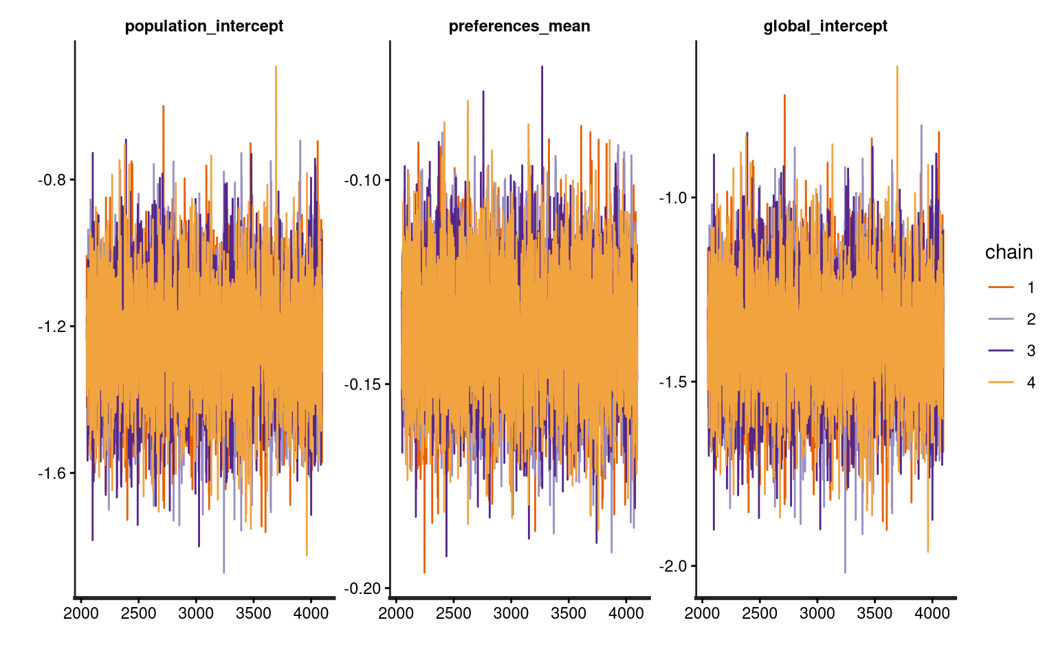
I spawned four chains here to get a more robust Gelman-Rubin statistic (\(\hat{R}\)), and fewer iterations than above because the sampler seems to find a minimum quickly. Nevertheless, sampling takes long, but is bareable (about 5 minutes on my machine).
post-hoc inspection
Issues would be easily visible on the traceplot, though these look good:
traceplot(model_fit, pars = c("population_intercept", "preferences_mean", "global_intercept"))
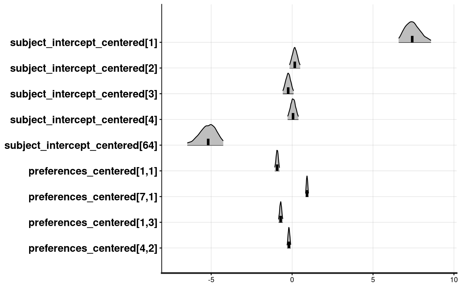
Visualizing the example effects memorized above:
plot(model_fit,
  show_density = TRUE, ci_level = 0.95,
  fill_color = "grey", fill_alpha = 0.6,
  pars = c(
           "subject_intercept_centered[1]", "subject_intercept_centered[2]",
           "subject_intercept_centered[3]", "subject_intercept_centered[4]",
           "subject_intercept_centered[64]",
           "preferences_centered[1,1]",
           "preferences_centered[7,1]",
           "preferences_centered[1,3]",
           "preferences_centered[4,2]"
           ),
)
ci_level: 0.95 (95% intervals)

outer_level: 0.95 (95% intervals)
We can extract specific measures, such as the “global intercept”.
# you could calculate your own stuff on the traces as follows
# (note that tuning/warmup are not included)
# population_level_intercept <- mean(as.data.frame(extract(model_fit))$population_intercept)
global_intercept <- mean(as.data.frame(extract(model_fit))$global_intercept)
global_intercept
[1] -1.375275
And we can extract the centered preference matrix, in the usual, clumsy R way.
preference_indexvector <- sapply(1:n_weekdays,
  FUN = function (j) sapply(
    1:n_brothels,
    FUN = function (i) sprintf("preferences_centered[%i,%i]", j, i)
  )
)

preferences_summary <- as.data.frame(summary(
  model_fit,
  pars = as.vector(preference_indexvector),
  probs = c()
)$summary)$mean


coeffs <- t(matrix(preferences_summary, ncol = n_weekdays, nrow = n_brothels))
rownames(coeffs) <- weekdays
colnames(coeffs) <- brothels


# comparison might not be fair if we would not center the reference
reference_logit_preferences_centered <- reference_logit_preferences - mean(reference_logit_preferences)

knitr::kable(coeffs - reference_logit_preferences_centered)
| The Velvet Hideaway | The Secret Garden | The Rosewood Retreat | Whispers & Lace | |
|---|---|---|---|---|
| Monday | -0.1562719 | -0.0822176 | 0.0611819 | 0.0410818 |
| Tuesday | -0.0214147 | 0.1038923 | -0.0165143 | -0.0168583 |
| Wednesday | 0.0014667 | -0.2974546 | -0.1412815 | -0.1233498 |
| Thursday | -0.0880503 | -0.0015510 | -0.0444559 | -0.0166098 |
| Friday | -0.0467117 | 0.0345246 | 0.1199643 | 0.0109021 |
| Saturday | 0.0445239 | 0.0769581 | 0.1388842 | 0.1230229 |
| Sunday | 0.0422637 | 0.1051565 | 0.0555122 | 0.0934060 |
plot(coeffs)
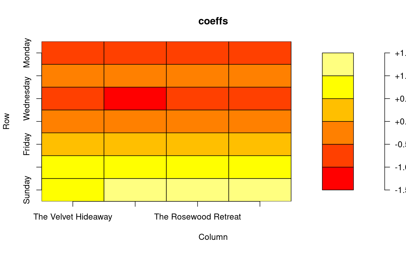
The model result is reasonably close to the true values, for most of the preference matrix, although the centering and separation of global preference baseline is different from the data generation process.
We were even able to cope with a problem of indetifiability, which I re-iterate out of fascination:
Despite all the efforts, some values are off. Think, for example, of the Pimp and Priest. We must conclude:
None of the models yielded exact results. We created an enormous, balanced sample, so this has little to do with the sample size demand of binary outcomes.
Instead, and especially for real experiments, we must conclude that no model can cover the real data. I would argue that this is always the case.
Though “only a model” (repeat the mantra!), it’s useful, anyways.
comparison to formula notation
Above (Section 6.4), I presented the formula visit ~ (1|brothel:weekday) + (1|subject), which worked reasonably well.
I must admit that this surprised me.
However, that formula implicitly also has to allocate the intercept to different factors, and it is not explicit about this.
Thus, how this formula handles identifiability remains opaque to the user, which is a problem. Also, I would prefer to also have the derived, centered results that I got with Stan.
Stan is more extensible: I could easily construct hierarchical effects for brothels (an “average brothel intercept”), or model the weekdays as sampled from a Circular Normal. Be creative!
However, keeping its limitations in mind, the formula syntax should be okay for everyday use and especially explorative modeling.
I think the go-to strategy are quick explorative results from lme4 or Python::statsmodels, and subsequently refining models in all details with Stan or its derivatives.
Interpretation of Intercepts (\(IoI^{TM}\))
Our specific model is, in fact, only intercepts. What does it tell us about suitors, weekdays, and brothels?
First thing to note is that we left planet earth and moved to logit space, which complicates interpretation.
A relative comparison of effects is valid (see the oggLods() function above for inverse logit transformation).
Both the subject intercepts and the preference matrix are centered, and so we get relative preferences. This means that we could say which weekday brings the most customers, on average. We could compare brothels, in all desired detail. And we could do all of that “per customer”.
I will limit interpretation to these more general capabilities, since the data was simulated anyways.
Comparing the simulation and the model outcome is useful to evaluate whether, keeping our assumptions in mind, the model can in principle recover the effects we expect.
I gave you the subsample function above to work on gradually changing sample sizes for power analysis, which I will skip for this already long text.
For the same reason, I will skip the vast topics of prior and posterior checks, model comparison, model “hygiene”; I covered some of those in my thesis (Ch. 4, p. 90).
TL;DR: Lessons Learned on Statistics
Take-Home Messages
This tutorial documents my random walk exploration of a “lattice model” of customer preferences (the preference matrix is a lattice), which is a type of “hierarchical overlapping multifactor model”, as the pro’s call it.
Some rather basic and more advanced take-home messages for me.
- Simulate your data before doing an experiment. This is good for conceptual exploration and power analysis, and best done before going to the field.
- While in exploration, introduce outliers and note down some more or less prominent known effects to check whether your model recovered the expected parameters.
- When Wilkinson notation (i.e. formulas) is sufficient, I tend to not use quick (plain RMSE optimizer) tools for model formula exploration: MCMC sampling is a major time and energy burden. You can happily use
stats::glmorlme4:glmeruntil you have a model that makes sense. - Interaction terms cover a specific relation of parameters, and must be used correctly. In particular, use
a*bwith caution, since it models every possible slope combination. - The
brms::make_stancode(formula)function might be the most powerful function of the wholebrmspackage. If only model code would be readable. Generally, in my personal opinionbrmscombines the intransparency of formulas with the sluggish sampling of Stan; the “worst of both worlds”. - In most cases, formulas do not get you far: it is preferrable to define stan models, even if that requires significantly more trial-and-error for starters.
- A hierarchical model structure, which could even be applied to a factor matrix (not shown), can provide logical links between parameters and thereby facilitate sampling (e.g. in cases of low sample size) at the cost of shrinkage.
- There can be good models with only intercepts. In our case,
visit ~ (1|brothel:weekday) + (1|subject)should be an appropriate formula. - There can be issues of identifiability and degeneracy. Auxiliary data might help to tip the sampler balance.
- Isolation and aggregation of mean preference and subject intercepts (“random effect”) converted our model results to relative preferences: which day/brothel did the customers prefer more or less, relative to their preference intercept? How do subjects compare to each other?
- There exist very few good models which simply work as you would expect. There exist bad models with perfectly plausible and exciting outcome: they are wrong because they do not mirror the data generating process, or because explanatory parameters are omitted (e.g. suitor age). There exist ugly models which do not sample well because they suffer (computational) degeneracy.
- The likelihood that your model is correct is exactly zero, for all practical purposes. Be humble in reporting.
Your models are wrong!
This last point is an important one, so allow me to elaborate a bit.
In the present example, data was simulated, and we knew the outcome.
Would you have guessed the correct model structure if I had not told you?
Even seeing the data generating code chunk above, would you have used the multiple intercept model, or turned to more common model formulas like y~a+bx?
And, depending on your answer: why? Maybe because you read another tutorial using a different formula? Maybe because you modeled interaction terms on different experiments in the past? Maybe because you did not carefully read the model formula documentation (I am guilty of this myself, but luckily never used forumlas).
There are an unnegligible degree of habit and ex post rationalization in model selection.
Transfer this to the uncomfortable situation of a real experiment. You cannot know the correct formula. There are some logical constraints to the space of all possible models. Sometimes you cannot sample the logically plausible model.
As a corollary, rigorously applying the logic of scepticism, we must conclude that all our models are most certainly wrong.
Can we do anything about it? No. However, we can acknowledge that our statistical results are just the findings derived from the models we apply.
We do not discover the truth. We apply models to a degenerate snapshot of the truth, and elaborate on plausible parameters.
This acceptance of degeneracy allows for a more humble way of reporting your results, more careful and balanced interpretation, and more to-the-point writing. As an exaggerated example, instead of writing
“Our extraordinary data set shows unquestionably (\(p<0.01\)) and for the first time in human history we know that customers prefer visiting brothels on Saturday…”
We could write along the lines of
“The limited sample we experimentally obtained, instructing a model which considered relative weekday-, brothel-, and subject effects, provides evidence that customers prefer Saturday over Monday (by \(xy %\)) for brothel visits.”
It is all in the formulation. Dare to show more schientific humility8!
Final Thoughts
I briefly went to Aarschotstraat on the day I started writing this article, at mid-afternoon, to catch the graffiti photos displayed above. Objectively, it is a disgusting place. At the entrance close to the station, there were some stinking tin urinals where old man queued constantly to piss. The street was crowded; the obvious gender bias you would expect. Worn old men who could be the fathers of the storefront ladies. Groups of young lads who could be the ladies’ sons. No single fairytale prince on his horse.
I chose the catchy example less to make a statistics tutorial more interesting, and more to initiate a thought process. To state it clearly, I do not feel entirely comfortable bringing up the topic of prostitution. My intention is not to trivialize it. On the other hand, I do not think that sex or sexual urges are shady, or immoral; they are normal. Still, every morning my train passes by, I feel pity for these women. Mostly because of their customers, and the work circumstances.
I think the recent law change in Belgium is a good initiative, if it can be implemented seamlessly. And, maybe most of all, I think that for a society as a whole, it is bad to conceal the topic of prostitution, as we did conceal the topic of sexuality for too long. It is worth talking about.
Denn die einen sind im Dunkeln Und die andern sind im Licht. Und man sieht nur die im Lichte Die im Dunkeln sieht man nicht.
(Bertold Brecht/Kurt Weill, “Dreigroschenoper”)
Notes and References
Further Reading:
- Stan Syntax Crash Course: https://www.sumsar.net/files/posts/2017-bayesian-tutorial-exercises/stan_cheat_sheet2.12.pdf
- Stan “unboxing”: https://www.alexpghayes.com/post/2018-12-24_some-things-ive-learned-about-stan/
- Identifiability and Degeneracy: https://betanalpha.github.io/assets/case_studies/identifiability.html#52_Additive_Degeneracy
- Degeneracy in Lattice Models: https://betanalpha.github.io/assets/case_studies/factor_modeling.html#35_Residual_Degeneracies
- Multilevel Models in Stan: https://willhipson.netlify.app/post/stan-random-slopes/varying_effects_stan/
- Multinomial Logit Models: https://eleafeit.com/posts/2021-05-23-parameterization-of-multinomial-logit-models-in-stan/
- History of Formula Notation https://stats.stackexchange.com/questions/284913/the-origin-of-the-wilkinson-style-notation-such-as-1id-for-random-effects-in/285026#285026
Thank you for reading!
-
Ioanna kindly offered to make her data available, but I do not think this is necessary. The hypothetical example used herein is equally illustrative. ↩︎
-
Betancourt (2021): “Impact Factor”. https://betanalpha.github.io/assets/case_studies/factor_modeling.html ↩︎
-
Side rant about the online R documentation: it is sponsored by “datacamp”, and the url has a static version in it. ↩︎
-
Wilkinson and Rogers (1973): “Symbolic Description of Factorial Models for Analysis of Variance” https://doi.org/10.2307/2346786 ↩︎
-
Wilkinson and Rogers (1973): “Symbolic Description of Factorial Models for Analysis of Variance” https://doi.org/10.2307/2346786 ↩︎
-
Trace plots, as everyone knows, should look like “hairy caterpillars”. ↩︎
-
I discovered this strategy on another one of the excellent blog posts by Michael Betancourt (2020): “Identity Crisis”. https://betanalpha.github.io/assets/case_studies/identifiability.html#52_Additive_Degeneracy ↩︎
-
Hoekstra and Vazire (2021): “Aspiring to greater intellectual humility in science”. Nat Hum Behav 5, 1602–1607. https://doi.org/10.1038/s41562-021-01203-8 ↩︎